Data science/ML/AI

▎Natural Language Processing (NLP)

Natural Language Processing (NLP) is a subfield of artificial intelligence that deals with the interaction between computers and human languages. The goal is to enable machines to understand, interpret, and generate human language in a valuable way.

▎Key Areas of NLP

1. Text Preprocessing
– Tokenization: Splitting text into words, phrases, or other meaningful elements.
– Normalization: Converting text to a standard format (e.g., lowercasing, removing punctuation).
– Stopword Removal: Filtering out common words that may not contribute significant meaning (e.g., "and", "the").
– Stemming and Lemmatization: Reducing words to their root forms.

2. Text Representation
– Bag of Words (BoW): A simple representation where text is represented as the frequency of words.
– TF-IDF (Term Frequency-Inverse Document Frequency): A statistical measure that evaluates the importance of a word in a document relative to a corpus.
– Word Embeddings: Techniques like Word2Vec, GloVe, and FastText that represent words in continuous vector space, capturing semantic relationships.

3. Language Models
– N-grams: Probabilistic models that predict the next item in a sequence based on the previous n items.
– Recurrent Neural Networks (RNNs): Neural networks designed for sequential data, often used for language modeling.
– Transformers: Advanced architecture that has revolutionized NLP, enabling models like BERT, GPT-3, and T5 to understand context better.

4. Text Classification
– Techniques for categorizing text into predefined categories (e.g., sentiment analysis, topic classification).
– Common algorithms include Naive Bayes, Support Vector Machines (SVM), and deep learning approaches.

5. Named Entity Recognition (NER)
– Identifying and classifying key entities in text (e.g., names, dates, locations).
– Often implemented using sequence labeling methods like Conditional Random Fields (CRFs) or neural networks.

6. Machine Translation
– Translating text from one language to another using statistical methods or neural networks.
– Notable models include Google's Transformer-based translation systems.

7. Question Answering and Chatbots
– Systems designed to answer questions posed in natural language.
– Chatbots utilize NLP techniques to understand user queries and provide relevant responses.

8. Sentiment Analysis
– Determining the sentiment expressed in a piece of text (positive, negative, neutral).
– Often involves feature extraction and classification techniques.

▎Tools and Libraries

1. NLTK (Natural Language Toolkit)
– A comprehensive library for working with human language data in Python.
– Provides easy access to many NLP tasks such as tokenization, stemming, and parsing.

2. spaCy
– An industrial-strength NLP library designed for performance.
– Supports tasks like part-of-speech tagging, named entity recognition, and dependency parsing.

3. Transformers by Hugging Face
– A library that provides pre-trained models for various NLP tasks based on transformer architecture.
– Allows easy fine-tuning and deployment of state-of-the-art models.

4. Gensim
– A library for topic modeling and document similarity analysis.
– Well-known for its implementation of Word2Vec.

What is Data Science?

▎t-SNE(t-distributed Stochastic Neighbor Embedding): A Deep Dive into Dimensionality Reduction

▎What is t-SNE?

t-SNE is a machine learning algorithm that helps visualize high-dimensional data by reducing it to two or three dimensions. This technique is particularly useful for visualizing complex datasets, such as those found in image recognition, text analysis, and bioinformatics.

▎Why Use t-SNE?

When dealing with high-dimensional data (like images with thousands of pixels or text represented by numerous features), it can be challenging to understand the underlying structure and relationships within the data. t-SNE helps by:

1. Preserving Local Structure: It keeps similar data points close together in the lower-dimensional space, which makes it easier to identify clusters or groups.

2. Revealing Global Structure: While it focuses on local relationships, t-SNE can also help highlight the overall distribution of the data.

3. Intuitive Visualization: The result is often visually appealing and interpretable, making it easier for analysts to communicate findings.

▎How Does t-SNE Work?

The algorithm works in two main steps:

1. Probability Distribution in High Dimensions: For each data point, t-SNE computes probabilities that represent the similarity between points based on their distances. It uses a Gaussian distribution to model these probabilities.

2. Probability Distribution in Low Dimensions: It then tries to find a lower-dimensional representation of the data that maintains these similarities as closely as possible. This is done using a Student's t-distribution to compute probabilities in the lower-dimensional space.

The algorithm minimizes the divergence between the two probability distributions using a technique called gradient descent.

▎Key Parameters

• Perplexity: This parameter balances attention between local and global aspects of the data. A smaller perplexity focuses more on local structure, while a larger one considers more global relationships.

• Learning Rate: This controls how much to change the representation during each iteration. A learning rate that's too high can lead to erratic results, while one that's too low may slow down convergence.

▎Example: Using t-SNE in Python

Here's a simple example of how to use t-SNE with the popular scikit-learn library on the famous Iris dataset:

import matplotlib.pyplot as plt
from sklearn import datasets
from sklearn.manifold import TSNE

# Load the Iris dataset
iris = datasets.load_iris()
X = iris.data
y = iris.target

# Apply t-SNE
tsne = TSNE(n_components=2, perplexity=30, random_state=42)
X_embedded = tsne.fit_transform(X)

# Plotting the results
plt.figure(figsize=(8, 6))
scatter = plt.scatter(X_embedded[:, 0], X_embedded[:, 1], c=y, cmap='viridis')
plt.title('t-SNE Visualization of Iris Dataset')
plt.xlabel('t-SNE Component 1')
plt.ylabel('t-SNE Component 2')
plt.colorbar(scatter, label='Species')
plt.show()

In this example, we load the Iris dataset, apply t-SNE to reduce its four dimensions down to two, and then visualize the results. The colors represent different species of iris flowers, showing how well t-SNE can separate them based on their features.

▎Limitations of t-SNE

While t-SNE is powerful, it has some limitations:

• Computationally Intensive: It can be slow for very large datasets due to its complexity.

• Non-Deterministic: Different runs can yield different results unless you set a random seed.

• Difficulty in Interpreting Distances: The distances in the lower-dimensional space do not have a direct interpretation; they are more about relative positioning than absolute distances.

▎Common Deep Learning Terms

1. Neural Network: A computational model inspired by the human brain, consisting of interconnected nodes (neurons) organized in layers.

2. Layer: A collection of neurons that process input data in a neural network; common types include input layers, hidden layers, and output layers.

3. Activation Function: A mathematical function applied to the output of each neuron, introducing non-linearity into the model; common examples include ReLU, sigmoid, and tanh.

4. Forward Propagation: The process of passing input data through the network to obtain an output prediction.

5. Backpropagation: An algorithm used to update the weights of a neural network by calculating the gradient of the loss function with respect to each weight.

6. Epoch: One complete pass through the entire training dataset during the training process.

7. Batch Size: The number of training examples used in one iteration of model training; affects memory usage and training speed.

8. Learning Rate: A hyperparameter that controls how much to change the model's weights during training based on the gradient of the loss function.

9. Dropout: A regularization technique that randomly sets a fraction of neurons to zero during training to prevent overfitting.

10. Convolutional Neural Network (CNN): A specialized type of neural network designed for processing grid-like data, such as images, using convolutional layers.

11. Recurrent Neural Network (RNN): A type of neural network designed for sequential data, allowing information to persist across time steps; often used in natural language processing.

12. Long Short-Term Memory (LSTM): A specific type of RNN architecture that can learn long-term dependencies by using memory cells and gates.

13. Generative Adversarial Network (GAN): A framework consisting of two neural networks (generator and discriminator) that compete against each other to generate new data samples.

14. Transfer Learning: A technique where a pre-trained model is fine-tuned on a new, often smaller dataset to leverage learned features.

15. Loss Function: A measure of how well the model's predictions match the actual outcomes; commonly used functions include mean squared error and categorical cross-entropy.

16. Optimizer: An algorithm used to adjust the weights of a neural network during training to minimize the loss function; examples include Adam, SGD, and RMSprop.

17. Gradient Descent: An optimization algorithm used to minimize the loss function by iteratively updating model parameters in the direction of the steepest descent.

18. Overfitting: A modeling error that occurs when a neural network learns noise and details from the training data too well, resulting in poor performance on unseen data.

19. Underfitting: A situation where a neural network fails to capture the underlying trend in the training data, leading to poor performance on both training and test datasets.

20. Data Augmentation: Techniques used to artificially increase the size of a training dataset by creating modified versions of existing data points (e.g., rotating, flipping images).

Data Warehouse vs Data Lake vs Lake House vs Mesh

▎Data Visualization: The Art of Turning Numbers into Stories

Imagine you’re at a party, and someone starts talking about how many people prefer pizza over tacos.

They could throw out a bunch of numbers, and you might nod politely, but your eyes would probably glaze over.

Now, picture them pulling out a vibrant pie chart that slices up the preferences in colorful segments. Suddenly, it’s not just numbers; it’s a story! You can see who loves pizza and who’s all about those tacos at a glance.

▎Why Data Visualization Rocks

1. Instant Understanding: Humans are visual creatures. Our brains process images 60,000 times faster than text! A well-designed graph can convey complex information quickly and clearly. It’s like giving your audience a cheat sheet to the data.

2. Spotting Trends and Patterns: Ever tried to read a spreadsheet with thousands of rows? Yikes! But with a line graph, you can easily spot trends over time like that steady rise in your friend's pizza sales during the summer. 🍕📈

3. Engagement: A captivating visual grabs attention and keeps people interested. Think of infographics or interactive dashboards, they’re like the cool kids of the data world, making everyone want to join the conversation.

4. Decision-Making: Good visuals help stakeholders make informed decisions. Instead of drowning in data, they can look at a bar chart comparing sales across regions and see where to focus their efforts.

▎Tools of the Trade

There are some pretty awesome tools out there to create stunning visuals:

• Tableau: This is like the Swiss Army knife of data visualization. It’s user-friendly and lets you create interactive dashboards without needing to code.

• Matplotlib Seaborn (Python): If you’re into coding, these libraries let you craft beautiful graphs right from your Python scripts. Perfect for those who love to get hands-on with their data!

• D3.js: For web developers, D3.js is a JavaScript library that brings data to life using HTML, SVG, and CSS. You can create anything from simple charts to complex interactive graphics.

▎A Quick Example

Let’s say you want to visualize your weekly coffee consumption (because who doesn’t love coffee?). Instead of just listing out numbers, you could create a bar chart showing how many cups you drink each day:

import matplotlib.pyplot as plt

# Days of the week
days = ['Mon', 'Tue', 'Wed', 'Thu', 'Fri', 'Sat', 'Sun']
# Coffee cups consumed
cups = [2, 3, 4, 1, 5, 6, 3]

plt.bar(days, cups, color='brown')
plt.title('Weekly Coffee Consumption')
plt.xlabel('Days')
plt.ylabel('Cups of Coffee')
plt.show()

With this simple code, you’ve transformed boring numbers into a visual that tells a story about your caffeine habits!

▎Conclusion

Data visualization isn’t just about making pretty pictures; it’s about making data accessible and understandable. It helps you tell stories that resonate with your audience and empowers them to make decisions based on insights rather than just raw numbers. So next time you have data to share, think about how you can visualize it, your audience will thank you!

▎Machine Learning Basics

Machine Learning (ML) is a subset of artificial intelligence that enables systems to learn from data and improve their performance over time without being explicitly programmed.

▎Core Concepts

1. Types of Machine Learning:
– Supervised Learning: The model is trained on labeled data (input-output pairs). Common algorithms include:
▪️ Linear Regression
▪️ Decision Trees
▪️ Support Vector Machines (SVM)
– Unsupervised Learning: The model works with unlabeled data to find patterns or groupings. Common algorithms include:
▪️ K-Means Clustering
▪️ Hierarchical Clustering
▪️ Principal Component Analysis (PCA)
– Reinforcement Learning: The model learns by interacting with an environment and receiving feedback in the form of rewards or penalties.

2. Key Components:
– Features: Individual measurable properties or characteristics used as input for the model.
– Labels: The output variable that the model aims to predict (in supervised learning).
– Training Data: The dataset used to train the model.
– Test Data: A separate dataset used to evaluate the model's performance.

▎Machine Learning Workflow

1. Data Collection: Gather relevant data from various sources.
2. Data Preprocessing: Clean and prepare the data for analysis, including handling missing values and normalizing features.
3. Model Selection: Choose an appropriate algorithm based on the problem type.
4. Training: Fit the model to the training data.
5. Evaluation: Assess the model's performance using metrics like accuracy, precision, recall, and F1-score.
6. Hyperparameter Tuning: Optimize the model's parameters to improve performance.
7. Deployment: Implement the model in a real-world application.

▎Example: Supervised Learning with Scikit-Learn

Here's a simple example using Python's scikit-learn library to perform linear regression:

import numpy as np
import matplotlib.pyplot as plt
from sklearn.model_selection import train_test_split
from sklearn.linear_model import LinearRegression

# Sample data
X = np.array([[1], [2], [3], [4], [5]])
y = np.array([2, 3, 5, 7, 11])

# Split data into training and test sets
X_train, X_test, y_train, y_test = train_test_split(X, y, test_size=0.2, random_state=42)

# Create and train the model
model = LinearRegression()
model.fit(X_train, y_train)

# Make predictions
predictions = model.predict(X_test)

# Plot results
plt.scatter(X, y, color='blue', label='Data Points')
plt.plot(X_test, predictions, color='red', label='Predicted Line')
plt.legend()
plt.show()

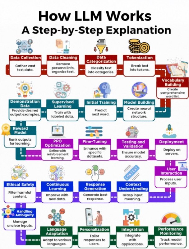
How LLMs Work: A Step by Step Explanation

▎Common Generative AI Terms

1. Generative AI: A type of artificial intelligence that can create new content, such as text, images, music, code, or videos, based on patterns learned from existing data.

2. Large Language Model (LLM): A deep learning model trained on massive amounts of text data, capable of understanding, generating, and manipulating human language. Examples: GPT-3.5, GPT-4, ChatGPT, Claude.

3. Tokens: The basic units of text that LLMs process. They can be words, sub-word units, or punctuation, and are used to break down input text.

4. Context Window: The maximum number of tokens an LLM can consider at once when processing input and generating output. A larger context window allows for longer conversations and more complex prompts.

5. Prompt: The input text or instructions given to a Generative AI model to elicit a specific response or output.

6. Prompt Engineering: The art and science of crafting effective prompts to guide Generative AI models to produce desired outputs, optimizing for accuracy, relevance, and style.

7. Zero-Shot Prompting: Asking an LLM to perform a task it hasn't been explicitly trained on, relying on its general knowledge and understanding of language.

8. Few-Shot Prompting: Providing an LLM with a few examples of input-output pairs within the prompt itself to demonstrate the desired task and improve performance.

9. Chain-of-Thought (CoT) Prompting: Encouraging an LLM to generate step-by-step reasoning before arriving at a final answer, improving performance on complex tasks.

10. Temperature: A parameter that controls the randomness of an LLM's output. Higher temperatures lead to more creative but potentially less coherent responses, while lower temperatures yield more focused and deterministic outputs.

11. Hallucination: When a Generative AI model produces incorrect, nonsensical, or fabricated information that is presented as factual.

12. Fine-tuning: The process of further training a pre-trained LLM on a smaller, specific dataset to adapt it to a particular task or domain.

13. Retrieval Augmented Generation (RAG): A technique that enhances LLMs by retrieving relevant information from an external knowledge base before generating a response, grounding the AI in factual data.

14. Embeddings: Numerical representations (vectors) of text, images, or other data that capture semantic meaning, allowing AI models to understand relationships between different pieces of information.

15. Latent Space: An abstract, multi-dimensional space where Generative AI models represent and manipulate data. The process of generating content involves navigating this space.

16. Diffusion Models: A class of generative models, popular for image generation, that work by gradually adding noise to data and then learning to reverse the process to create new data.

17. Generative Adversarial Network (GAN): A framework consisting of two neural networks (a generator and a discriminator) that compete against each other to produce highly realistic synthetic data.

18. Multimodal AI: Generative AI models capable of understanding and generating content across multiple modalities, such as text, images, audio, and video.

19. Transformer Architecture: The foundational neural network architecture that powers most modern LLMs, known for its ability to process sequential data and capture long-range dependencies.

20. Content Moderation: Processes and tools used to ensure that AI-generated content adheres to safety guidelines, ethical standards, and legal requirements, preventing the creation of harmful or inappropriate material.

Data Pipeline Overview

🎭 The Deceiving Score: Accuracy vs. Precision/Recall (Imbalanced Data) 💡

Your model to detect a rare disease (1% prevalence) boasts 99% accuracy. Impressive? Not if it just says "NO DISEASE" to everyone! For imbalanced data, plain accuracy is a lie.


📈 The Problem: Imbalanced Data
Many real-world cases (fraud, disease, ad clicks) have a tiny "positive" class. A model predicting the majority class (e.g., "no disease") will have high accuracy but be useless for finding the rare events you care about.

📊 Beyond Accuracy: The Confusion Matrix
Break down predictions into:
• True Positives (TP): Correctly found the positive.
• True Negatives (TN): Correctly found the negative.
• False Positives (FP): Wrongly said positive (costly "false alarms").
• False Negatives (FN): Wrongly said negative (costly "missed opportunities").


🎯 The Right Metrics

• Accuracy: (TP+TN) / Total - Avoid for imbalanced data!
• Precision: TP / (TP + FP)
• Meaning: Out of all times it said "Positive," how many were truly positive?
• Use When: False Positives (FP) are very costly (e.g., wrongly flagging a healthy person as sick).
• Recall: TP / (TP + FN)
• Meaning: Out of all actual positives, how many did it catch?
• Use When: False Negatives (FN) are very costly (e.g., missing a real fraud, not detecting a tumor).
• F1-Score: Balances Precision and Recall.


🐍 Code Example: The 99% Accurate Lie

from sklearn.metrics import accuracy_score, precision_score, recall_score
import numpy as np

y_true = np.concatenate([np.zeros(990), np.ones(10)]) # 1000 samples, 1% positive

# Model 1: Always predicts '0' (no disease)
y_pred_bad = np.zeros(1000) 
print(f"Model 1 (Always No Disease):\n  Accuracy: {accuracy_score(y_true, y_pred_bad):.2f}")
print(f"  Precision: {precision_score(y_true, y_pred_bad, zero_division=0):.2f}") # 0.00!
print(f"  Recall: {recall_score(y_true, y_pred_bad):.2f}\n") # 0.00!

# Model 2: Catches 5 positives, 2 false alarms (Better!)
y_pred_better = np.zeros(1000)
y_pred_better[990:995] = 1 # 5 True Positives
y_pred_better[100:102] = 1 # 2 False Positives
print(f"Model 2 (Actually Catches Some):\n  Accuracy: {accuracy_score(y_true, y_pred_better):.2f}")
print(f"  Precision: {precision_score(y_true, y_pred_better, zero_division=0):.2f}") # 0.71
print(f"  Recall: {recall_score(y_true, y_pred_better):.2f}") # 0.50
# Model 2's accuracy might be slightly lower, but its Precision/Recall shows it's far superior!

🎯 Today's Goal (What you should do)
✔️ Recognize accuracy's flaw for imbalanced data.
✔️ Pick Precision when False Positives hurt most.
✔️ Pick Recall when False Negatives hurt most.
✔️ Understand what your model's mistakes truly cost.